Real Estate Analysis

DESCRIPTION :

• A banking institution requires actionable insights into mortgage-backed securities, geographic business investment, and real estate analysis.
• The mortgage bank would like to identify potential monthly mortgage expenses for each region based on monthly family income and rental of the real estate.
• A statistical model needs to be created to predict the potential demand in dollars amount of loan for each of the region in the USA. Also, there is a need to create a dashboard which would refresh periodically post data retrieval from the agencies.
• The dashboard must demonstrate relationships and trends for the key metrics as follows: number of loans, average rental income, monthly mortgage and owner’s cost, family income vs mortgage cost comparison across different regions. The metrics described here do not limit the dashboard to these few.

Dataset Description:

• Second mortgage                       : Households with a second mortgage statistics
• Home equity                               : Households with a home equity loan statistic
• Debt                                              : Households with any type of debt statistics
• Mortgage Costs                           : Statistics regarding mortgage payments, home equity loans, utilities, and property taxes
• Home Owner Costs                    : Sum of utilities, and property taxes statistics
• Gross Rent                                   : Contract rent plus the estimated average monthly cost of utility features
• High school Graduation            : High school graduation statistics
• Population Demographics        : Population demographics statistics
• Age Demographics                     : Age demographic statistics
• Household Income                    : Total income of people residing in the household
• Family Income                           : Total income of people related to the householder

Analysis Task:

• Importing pandas, numpy, seaborn, matplotlib.pyplot, seaborn libraries for analysis task.
• Figuring out the primary key and looking for the requirement of indexing.

Exploratory Data Analysis:

• Explore the top 2,500 locations where the percentage of households with a second mortgage is the highest and percent ownership is above 10 percent.
• Visualize using geo-map and keeping the upper limit for the percent of households with a second mortgage to 50 percent
• Use the following bad debt equation: Bad Debt = P (Second Mortgage ∩ Home Equity Loan) Bad Debt = second_mortgage + home_equity - home_equity_second_mortgage.

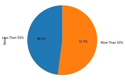
Pie Charts to show overall debt and bad debt

• Create Box and whisker plot and analyze the distribution for 2nd mortgage, home equity, good debt, and bad debt for different cities

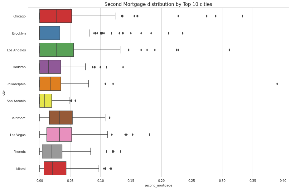
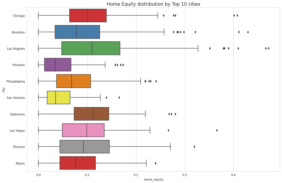
•Created a collated income distribution chart for family income, house hold income, and remaining income

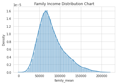
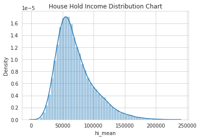
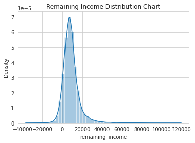
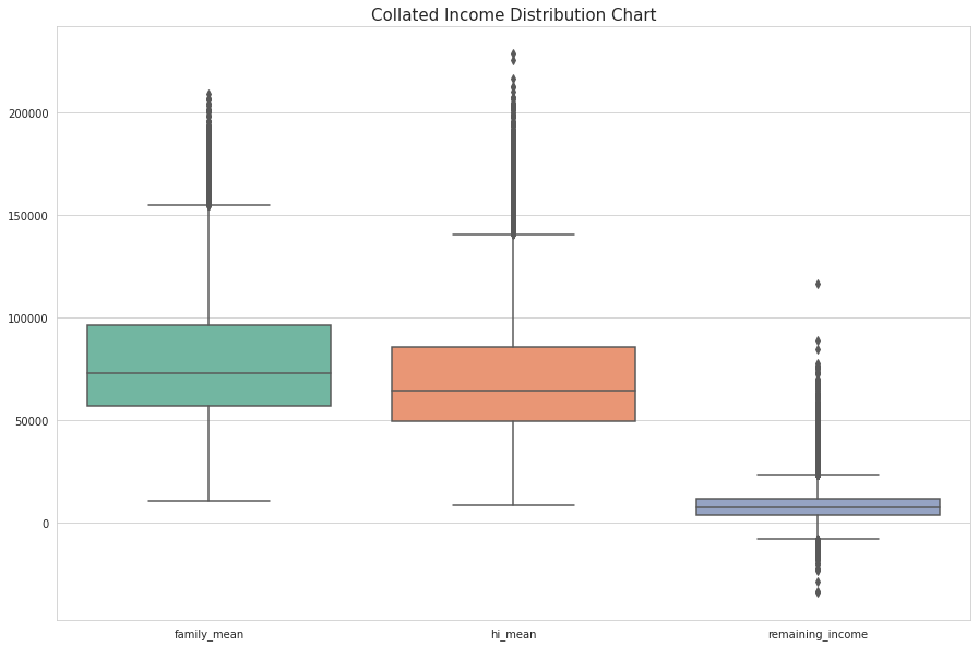
Collated Income Distribution Chart

•Performed EDA and came out with insights into population density and age. I have to derive new fields, and I have to make sure that the weight averages are accurate for measurements.

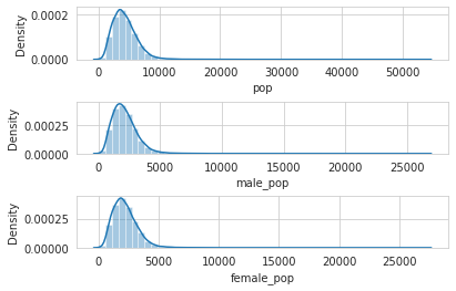
Density Charts

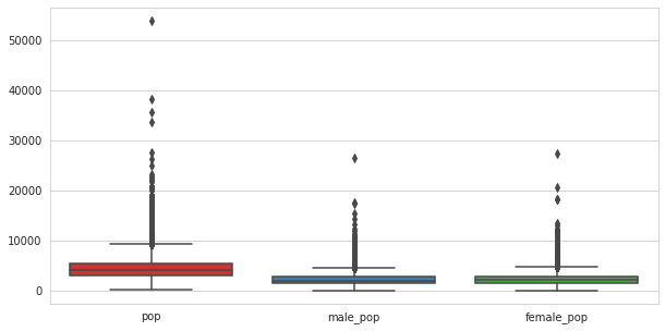
Box plot

•Used pop and ALand variables to create a new field called population density

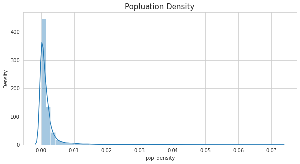
Population Density

•Used male_age_median, female_age_median, male_pop, and female_pop to create a new field called median age
•Visualize the findings using appropriate chart type

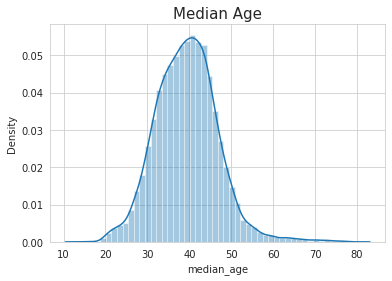
Median Chart

•Age of population is mostly between 20 and 60
•Majority are of age around 40
•Median age distribution has a gaussian distribution
•Some right skewness is noticed

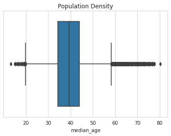
Population density with median age

•Analyze the married, separated, and divorced population for these population brackets
•Visualize using appropriate chart type
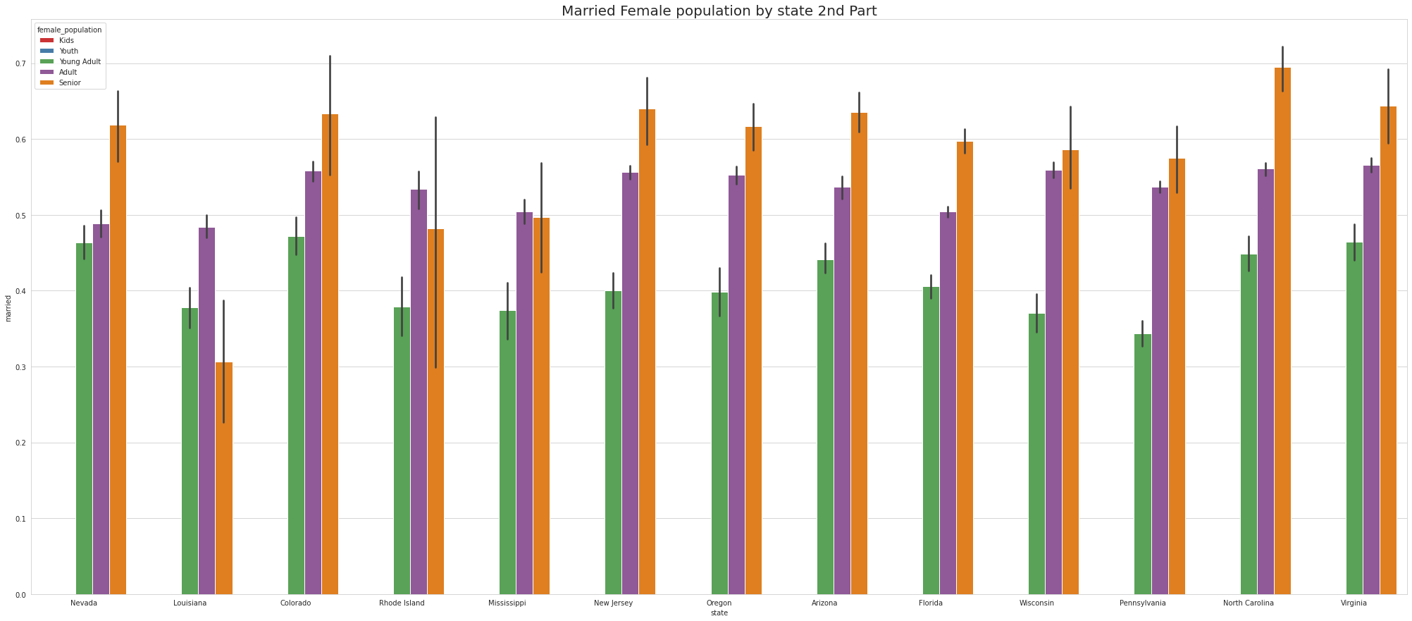
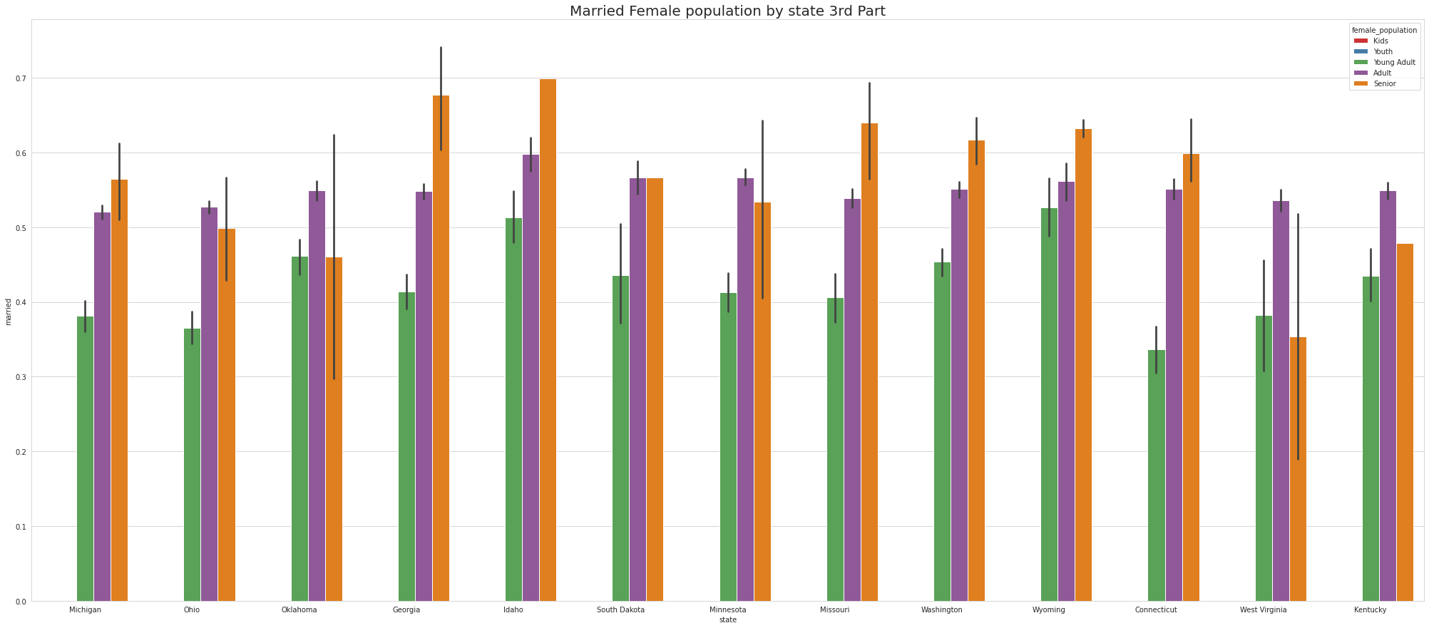
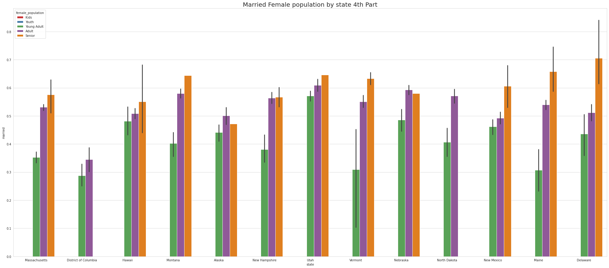
•To ease the visulaize we are splitting states into 4 part which means there are 52 unique states and we are divding 52 states by 4.So, one part of the splitting will contain 13 states.

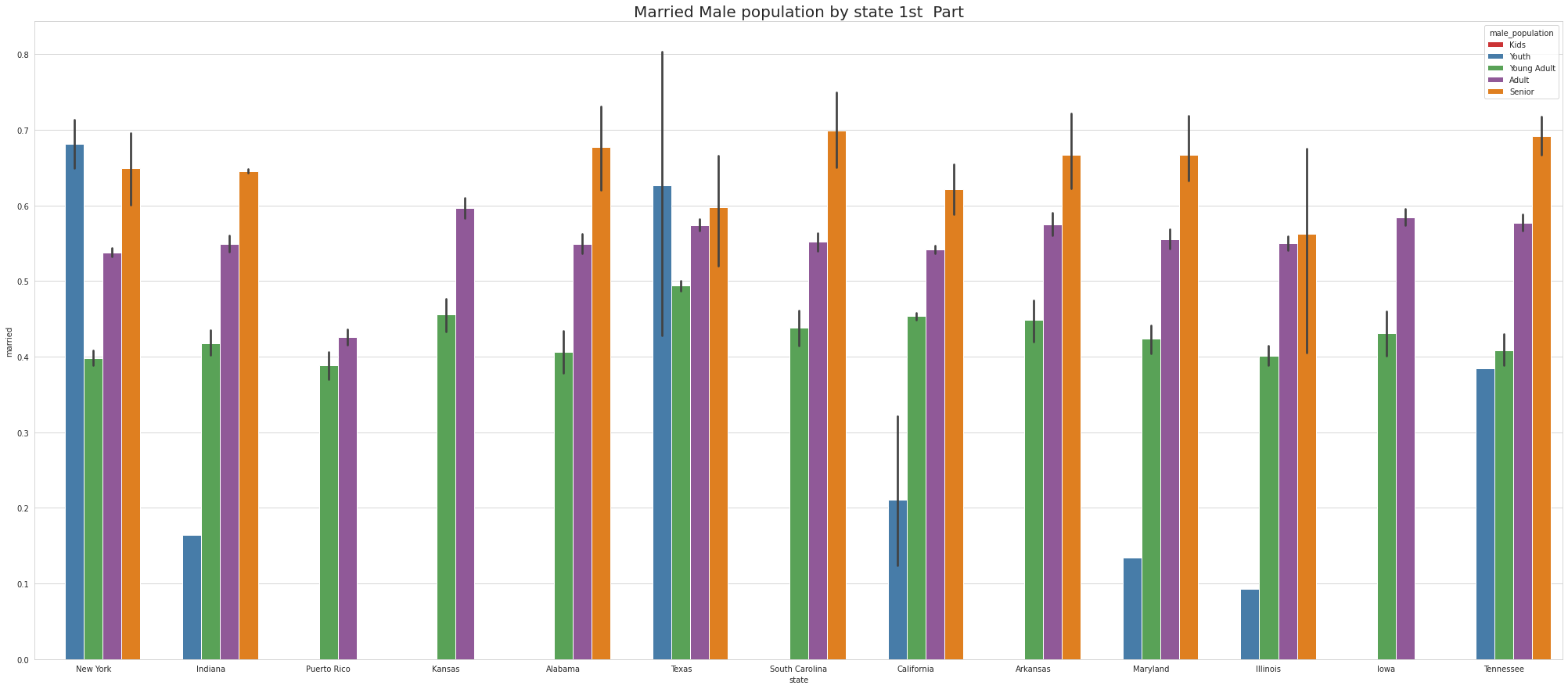
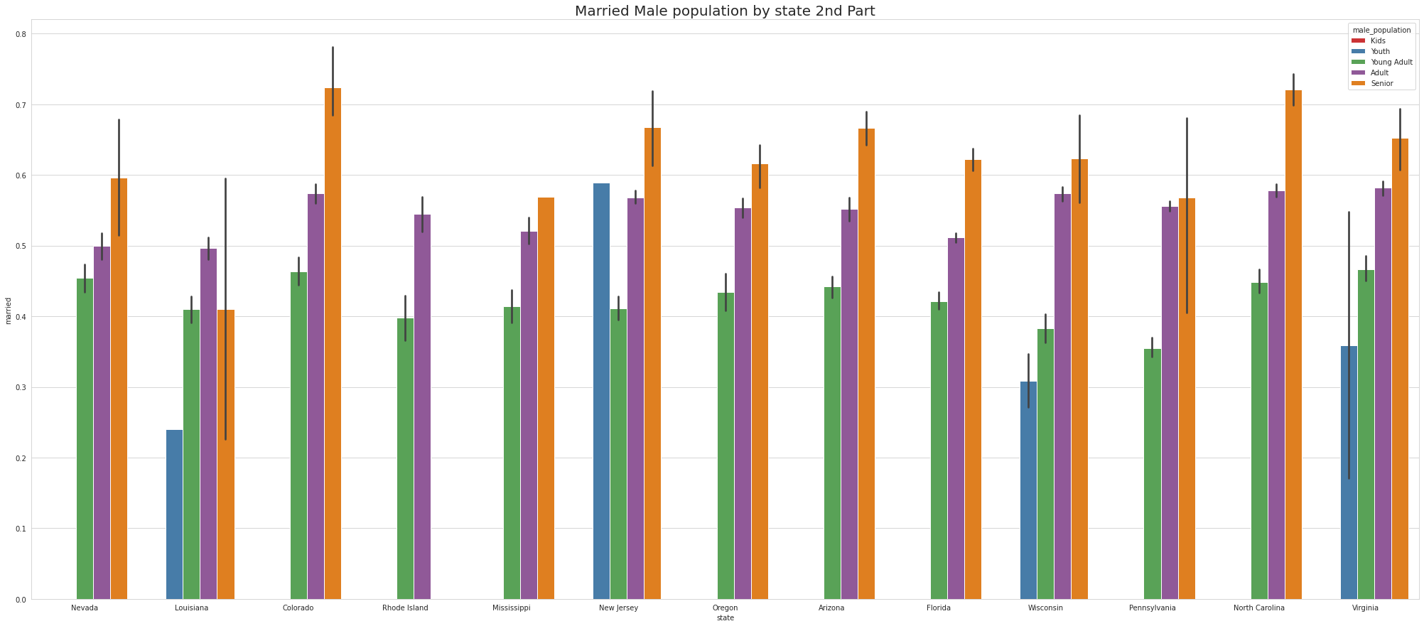
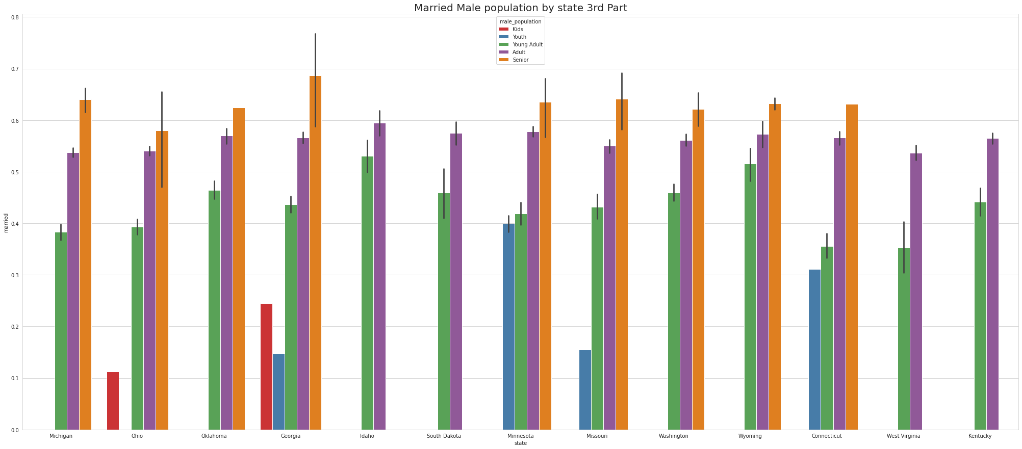
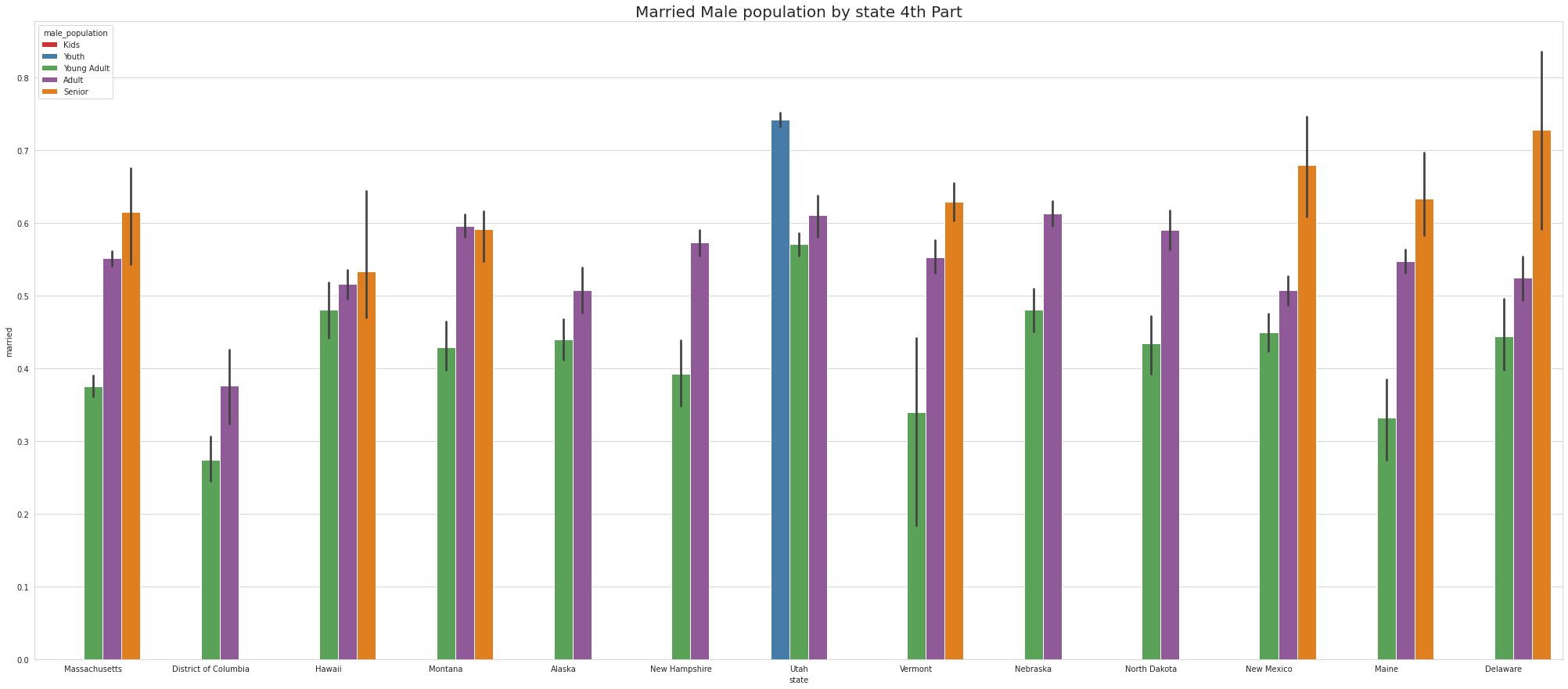
•Ohio & Georgia have Married Male KIDS

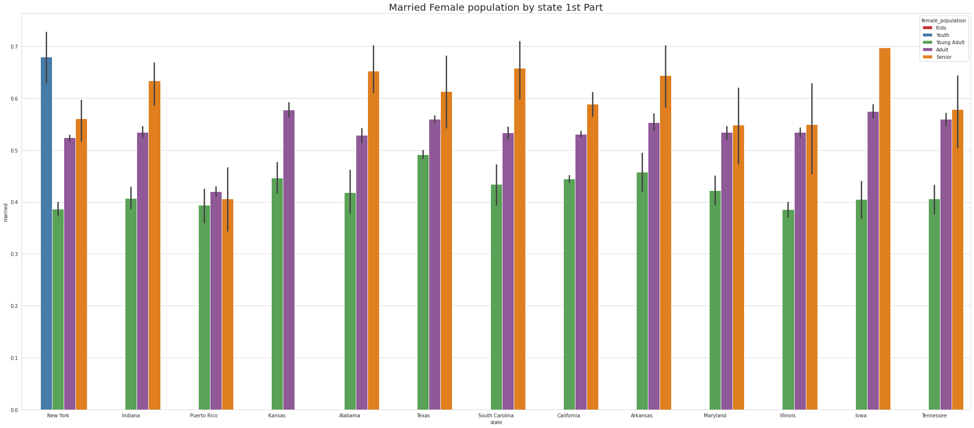
•Except NewYork no other states has youth

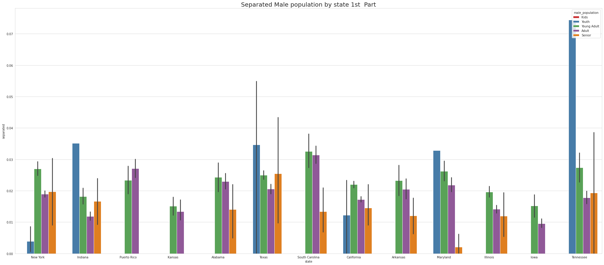
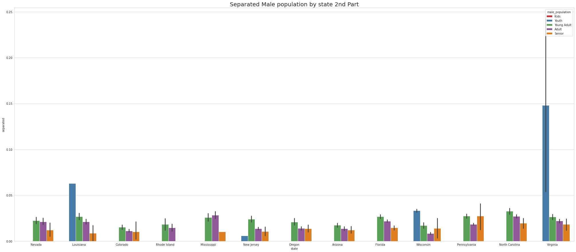
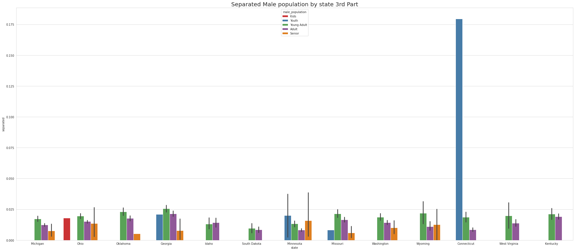
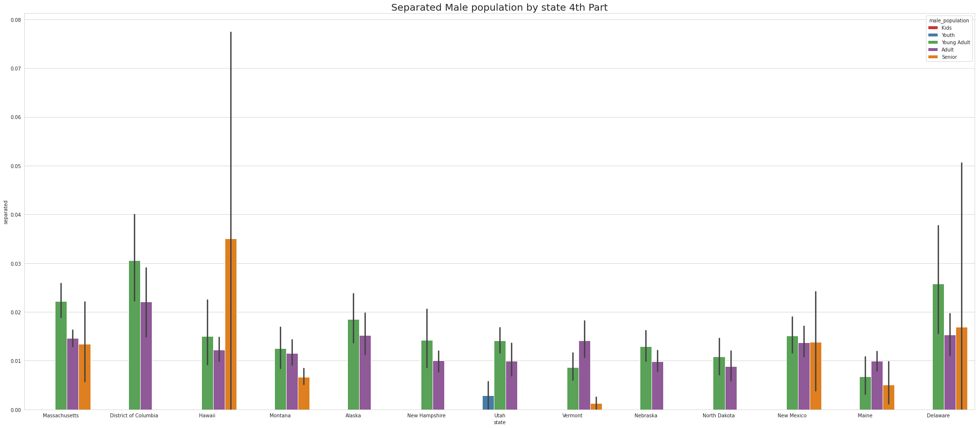
•Tennessee has Highest youth separated in 1st part, Virgina Has highest youth seperated in 2nd part and Connecticut has highest youth seperated in 3rd Part.

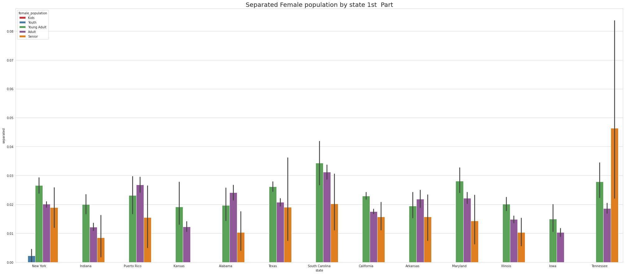
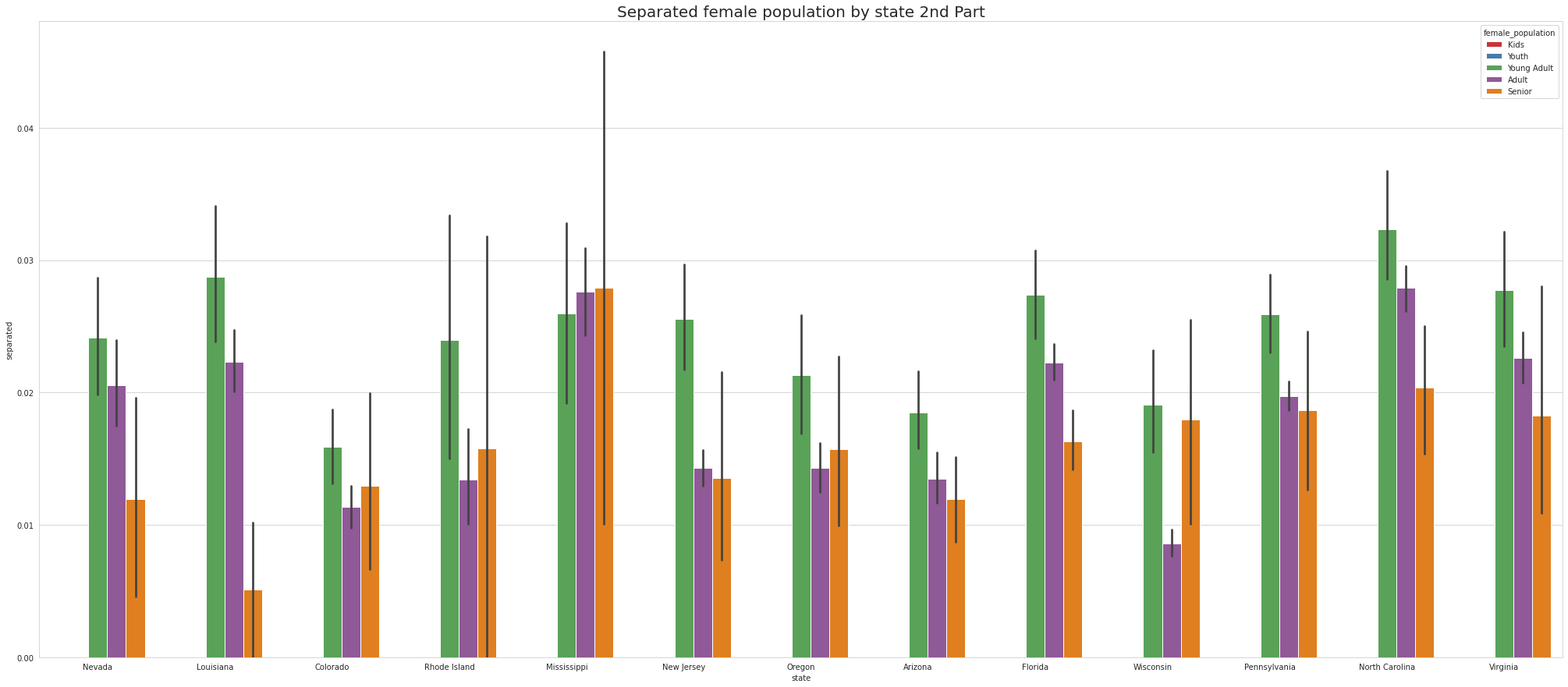
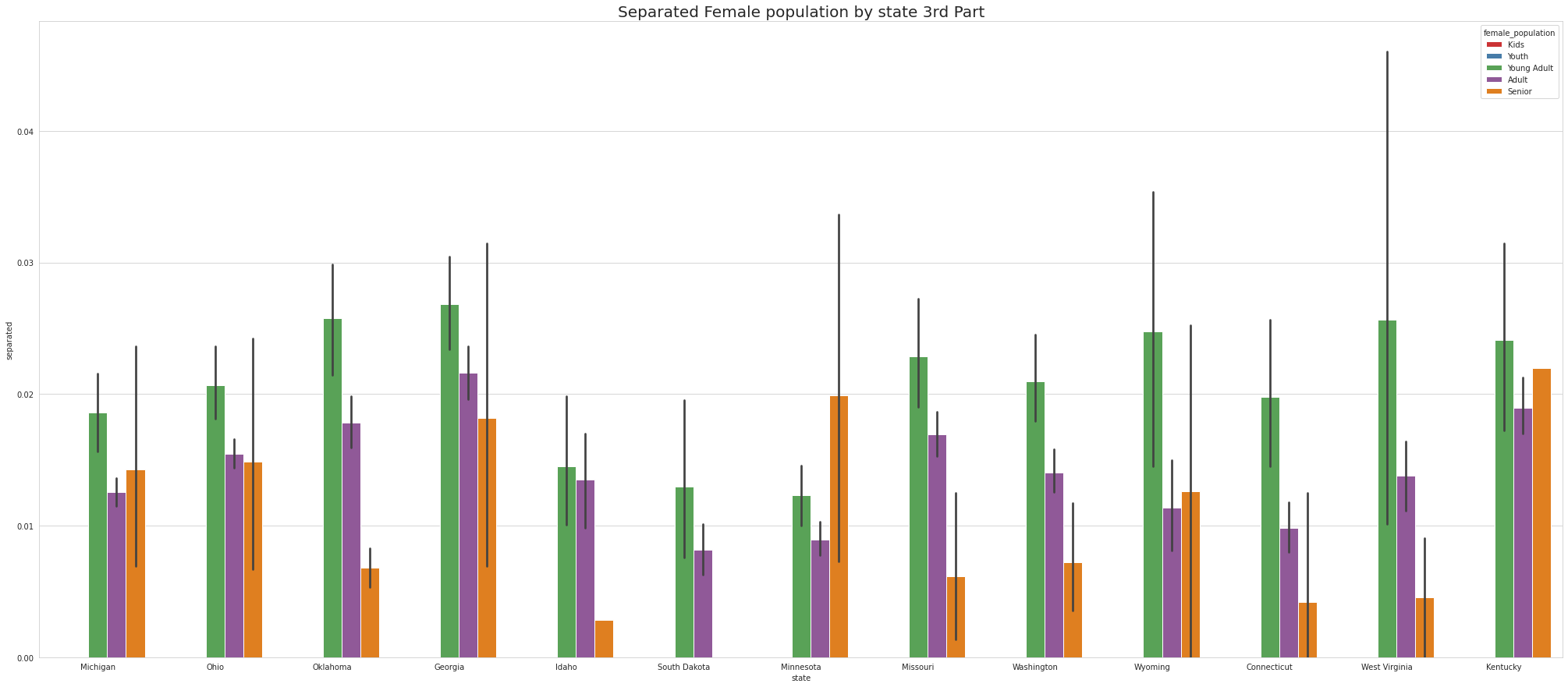
•Except for Newyork, No other state has Separated Female Youth population Tennessee has the Highest Separated Female Senior population

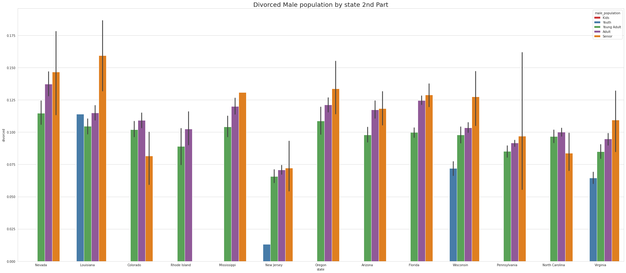
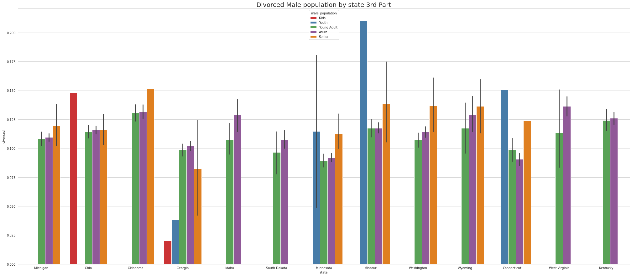
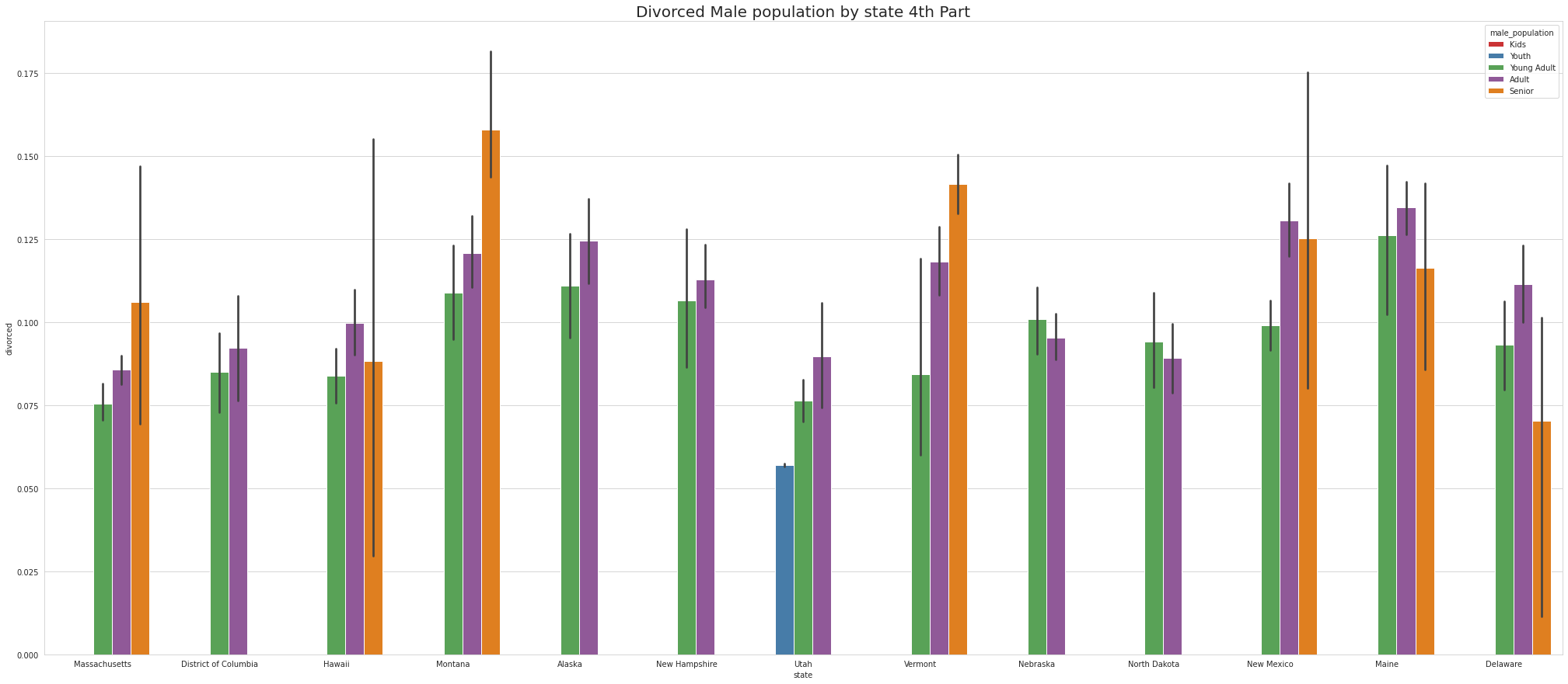
•Ohio has Largest number of Divorced Male KIDS.
•Missouri & Connecticut has Largest number of Divorced Male YOUTH.
•Maine, Indiana & Oklahoma has Largest number of Divorced Male YOUNG ADULTS.
•Arkansas, Maine, Neveda, Indiana & Oklahoma has Largest number of Divorced Male ADULTS.
•Louisiana, OKlahoma & Montana has Largest number of Divorced Male SENIORS

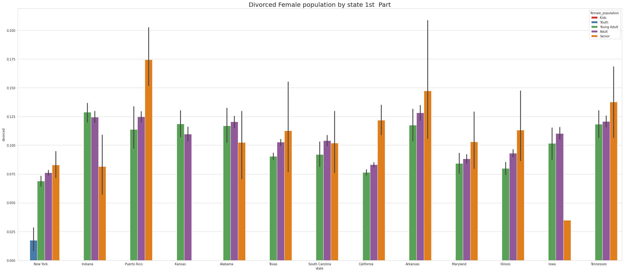
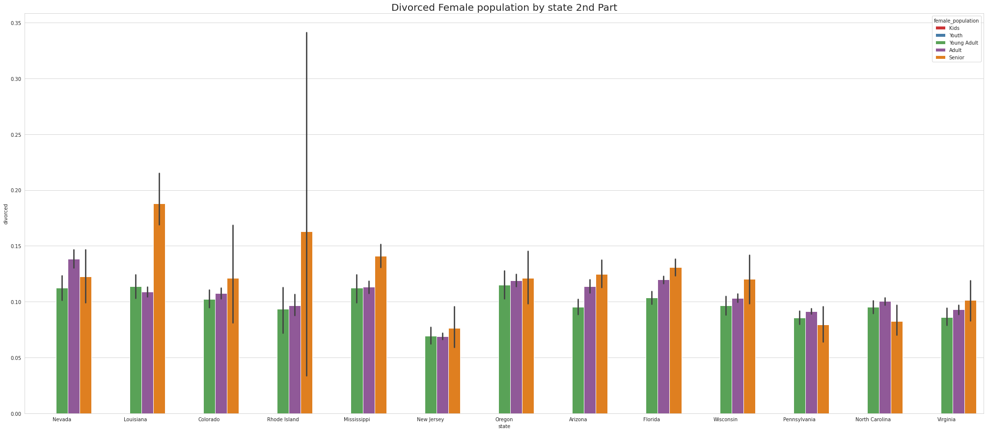
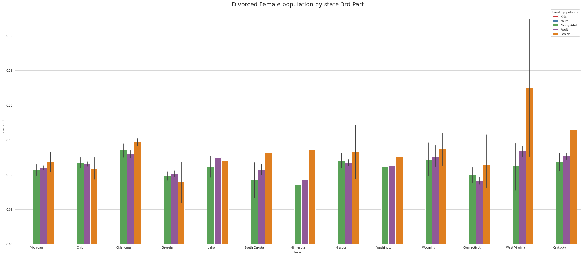
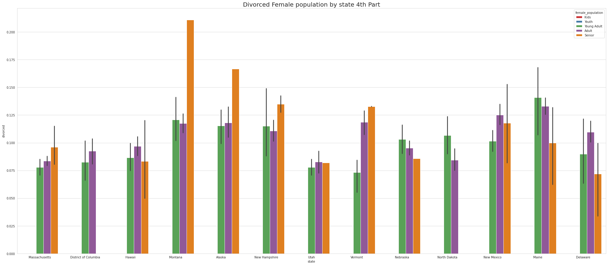
•Newyork is the only state that has Divorced Female YOUTH.
•Maine has Largest number of Divorced Female YOUNG ADULTS.
•Maine has Largest number of Divorced Female ADULTS.
•Montana has Largest number of Divorced Female SENIOR

Perform correlation analysis for all the relevant variables by creating a heatmap

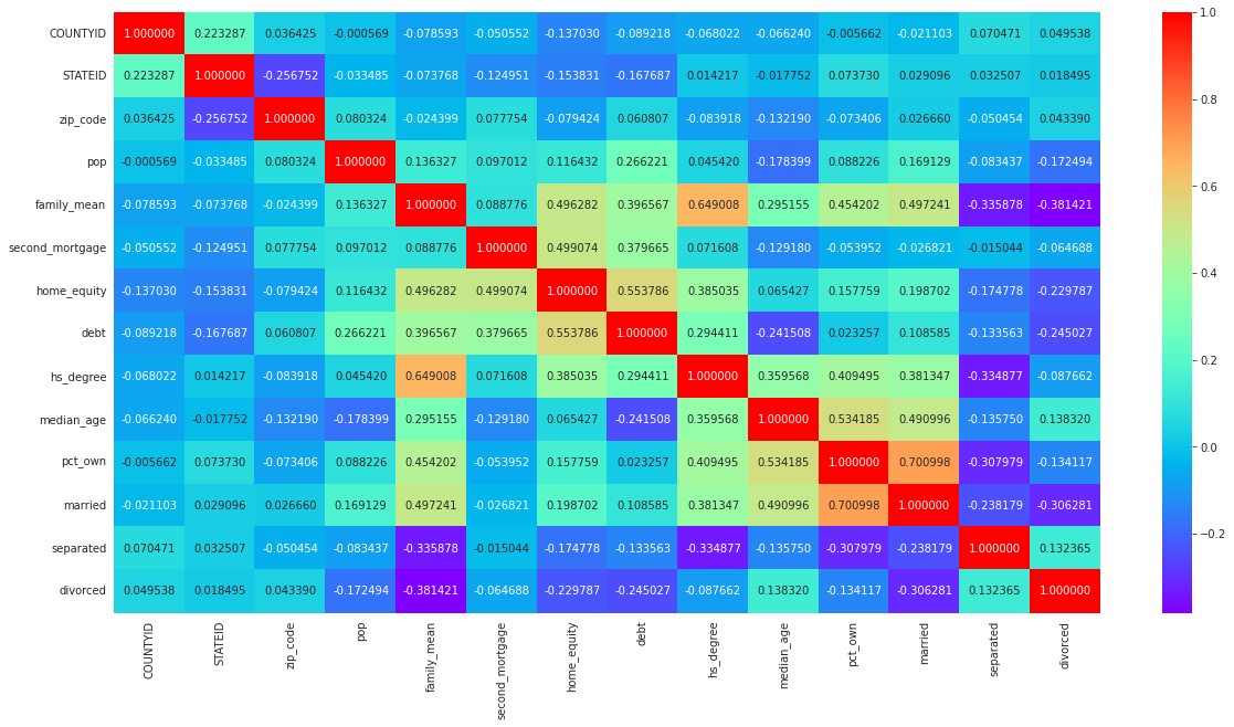
Correlation Matrix

•High positive correaltion is noticed between pop, male_pop and female_pop
•High positive correaltion is noticed between rent_mean,hi_mean, family_mean,hc_mean

Data Pre-processing:

•The economic multivariate data has a significant number of measured variables.
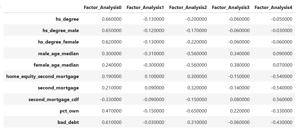
•The goal is to find where the measured variables depend on a number of smaller unobserved common factors or latent variables.
•Each variable is assumed to be dependent upon a linear combination of the common factors, and the coefficients are known as loadings.
•Each measured variable also includes a component due to independent random variability, known as “specific variance” because it is specific to one variable.
•Obtain the common factors and then plot the loadings.
•Use factor analysis to find latent variables in our dataset and gain insight into the linear relationships in the data.
•Following are the list of latent variables:

• Highschool graduation rates
• Median population age
• Second mortgage statistics
• Percent own
• Bad debt expense

•Chi-Square and P-Value is 9045268.678767936, 0.0
•Kaiser–Meyer–Olkin value is 0.21258179885097275

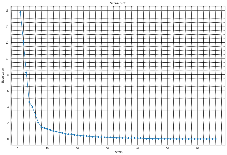
Plotting Eigen Values with Factor Values

• Highschool graduation rates

• Median population age
• Second mortgage statistics
• Percent own
• Bad debt expense

Data Modeling :

•Build a linear Regression model to predict the total monthly expenditure for home mortgages loan.

•Mean Absolute Error is 43.67
•Mean Squared Error is 4673.49
•Root Mean Squared Error is 68.36
•R2 Score is 0.99

•Regression Model with all dependent numeric variables at Nation level is giving R SQUARED metric of 99%. So skipping state level Regression Model
•Run another model at State level. There are 52 states in USA
•STATEID - 1

•Mean Absolute Error:11389503548.48
•Mean Squared Error:2.0908859553935737e+20
•Root Mean Squared Error:14459896110.95
•R2 Score:-410429821366382.56

•STATEID - 20

•Mean Absolute Error:246.6 •Mean Squared Error:84714.13 •Root Mean Squared Error:291.06 •R2 Score:0.63

•STATEID - 45

•Mean Absolute Error:8822908571370.76
•Mean Squared Error:1.553802280528196e+26
•Root Mean Squared Error:12465160570679.37
•R2 Score:-6.443994385547235e+20

•Ensure Multi-collinearity does not exist in dependent variables
•Dropped MultiCollinear variables and ran the Regression Model

•Mean Absolute Error:44.0
•Mean Squared Error:4787.23
•Root Mean Squared Error:69.19
•R2 Score:0.99

•We have achieved an R Squared value of 99% which is pretty close to 1.